The Comminution Energy Curves contain data from comminution circuits that process a wide range of commodities. All commodities can be compared equitably across most metrics because the mill performance is not influenced by the mineral being processed, but rather is determined by the material competence, circuit performance and grind size requirements. However, one metric is not comparable: the metal specific energy (the energy per unit metal recovered from the ore). This measurement was highlighted in the 2012 CEEC workshop as being of prime importance when investigating comminution energy efficiency. It is well known that “The most efficient way to break rock is not to break rock at all” - Dr Rob Morrison, JKMRC. Therefore, the most effective method for reducing comminution energy consumption is to remove low grade material prior to comminution, thereby reducing the amount of material that requires grinding. This process is commonly referred to as preconcentration or gangue rejection and can only be compared to other strategies if the energy intensity is measured as a function of the metal content of the ore, because this is the measure it directly acts upon. Additionally, the fineness of the grind is targeted to achieve a certain recovery of metal, therefore metal recovery can be an important indicator for comminution effectiveness, other key factors being relatively equal. Therefore, the metal specific energy intensity is an important parameter for the comminution energy curves, but comparing disparate commodities is complex and multifaceted.
The concept of copper equivalent production was used to present data for different commodities on the same graph. Metal equivalent calculations are common practice for polymetallic deposits and are especially popular in South America (Rendu, 2008). The copper equivalent production (Cue) is defined as the production of copper that would be required to obtain the same revenue. For simplicity, complex factors related to product quality, smelting and refining were not included in the analysis. Commodity prices are set by the market and are a balance of supply and demand. Therefore, using commodity prices as a comparison tool is likely to reflect the investment in mining at a specific time. However, the choice of the reference date for the commodity prices is important because it can influence a comparison, especially when relative prices between copper and other commodities vary significantly.
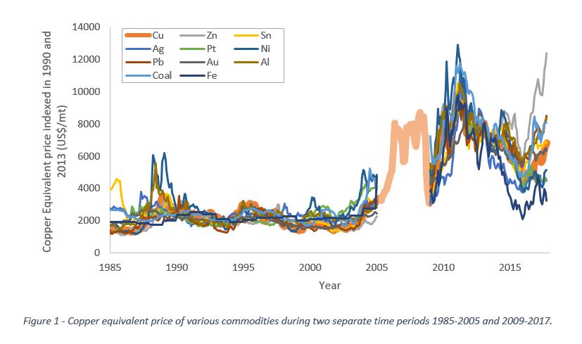
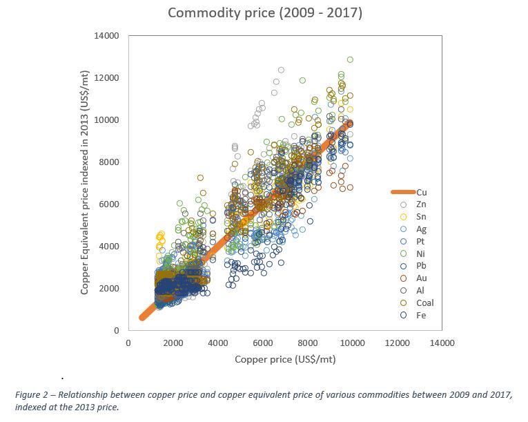
The prices for copper, gold, lead, zinc silver, tin, nickel, platinum, aluminium, coal and iron ore from 1960 to 2017 were sourced via the world bank. These commodities were chosen because they represented all the commodities covered in the energy curve database. Two date range regimes were studied, 1985-2005 and 2009-2017, because in these periods the commodity prices appeared to follow consistent trends. The copper equivalent price was determined for each commodity by using the prices recorded at a specific date. The sum of squared errors between the equivalent and actual copper prices were determined for all the commodities, and the date which corresponded to the lowest value was set to be the reference date. 1990 and 2013 were found to be the most effective reference dates for the first and second date ranges respectively. Figure 1 shows the copper equivalent price over the fitted ranges and Figure 2 shows the accuracy of the fit. What is clear from these plots is that the copper price variance generally tracks the other commodity prices well, but there are other factors that lead to deviations. For instance zinc out performed copper since 2013, but iron underperformed which has led to the copper equivalent price for zinc being 9000 $US/t more than iron ore in 2017.
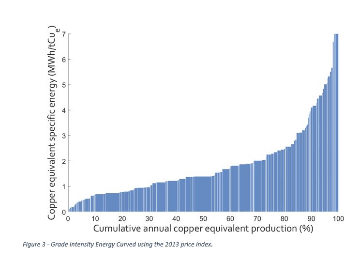
Copper equivalent production was used to produce the grade intensity energy curves. The 2013 commodity prices were used to calculate the copper equivalency, and the energy curve is shown in Figure 3.