The energy curve database incorporates comminution circuit data for 169 mines across 9 commodities. Although it is useful to compare all these data on the same curve, a mine may also want to visualise their performance against mines in the same commodity. However, the data has been submitted confidentially and isolating commodities in a traditional energy curve approach is likely to unintentionally make some mines obviously identifiable. Therefore, an approach has been developed to describe the shape and nature of the distribution, without displaying the raw data of each mine. In this way, the comminution energy intensity of different commodities can be explored.
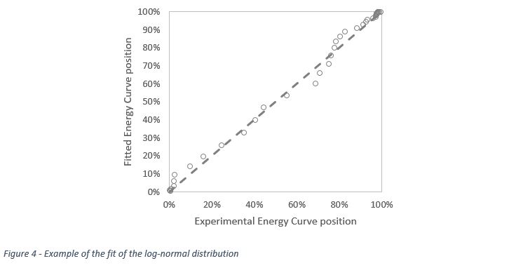
The first step was to find a mathematical function that adequately described the distribution. Individual commodities were isolated and Weibull, Normal, Beta, Gamma and log-normal functions were fitted to the energy curve distributions. The log-normal was found to provide the best fit to the distribution with the lowest standard error. Figure 4 shows an example of the close fit that is achieved with the log-normal distribution.
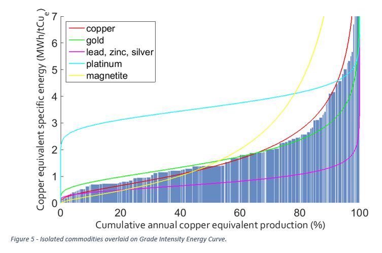
Utilising this method, individual distributions can be generated that represent each of the individual commodities in the Energy Curve database. These distributions can then be displayed overlaid on one of the full traditional Comminution Energy Curves. Figure 5 shows the results for six of these commodities: copper, gold, (lead, zinc, silver), platinum and magnetite. It is evident from these distributions that magnetite has a higher range of results and includes very high energy intensity figures. Whereas, lead, zinc, silver mines consumed significantly lower energy intensities possibly due to their consistently lower competence. Copper and gold are very close to the overall distribution, due to the large majority of the database focused on these commodities.
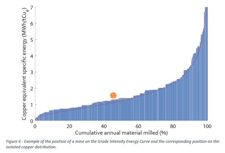
The isolation of individual commodities can be conducted on each of the Energy Curves included in the standard suite. The same methodology can be used to isolate other categories such as circuit type, geographical location or mine type. This kind of comparison lends itself to a flexible application embedded with the energy curve visualisation. Figure 6 shows the potential visualisation that could be utilised in this kind of approach. The ball shows the position of a particular mine on the complete energy curve. The line was drawn across to the isolated copper curve. This mine was close to the 42nd percentile on the complete energy curve, but above the 50th percentile of the isolated copper curve. Although this example is presented for copper, the differences are more stark for other commodities where the distribution is dramatically different from the standard energy curve. It allows mines to compare apples with apples, but showing the full database as required.